2  Computing Probabilities

There are many common families of probability distributions and we have discussed six so far. The discrete distributions include the discrete Uniform, Bernoulli, and Binomial. The continuous distributions include the continuous Uniform, Normal, and t.

This chapter provides a set of examples to show you how to compute probabilities from a few of these distributions in R.

2.1 Normal Distribution

R has four normal distribution functions: dnorm( ), pnorm( ), qnorm( ), and rnorm( ).

dnorm(x,mean,sd) probability density function (PDF) - input: x is the value at which you want to evaluate the normal PDF - output: a positive number since the PDF \(f(x)\) must be positive - example: evaluate \(f(x)\)

pnorm(q,mean,sd) cumulative distribution function (CDF) - input: q is the value for which you want to find the area below/above - output: a probability - example: compute \(P(X<q)\)

qnorm(p,mean,sd) quantile function - input: p is a probability - output: a real number since \(X\in(-\infty,\infty)\) - example: find the value \(q\) such that \(P(X<q)=p\)

rnorm(n,mean,sd) random number generator - input: n is the number of observations you want to generate - output: a vector of n real numbers - example: generate n independent \(N(\mu,\sigma^2)\) random variables

More information is also accessible in R if you type ?dnorm, ?pnorm, ?qnorm, or ?rnorm.

To learn how to use these functions, we’ll start with a few exercises on the standard normal distribution which is a normal distribution with mean 0 and standard deviation of 1. We will then move on to the more general \(N(\mu,\sigma^2)\) distribution.

2.1.1 Probability Density Function (dnorm)

When \(X\) is a continuous random variable, we know that \(P(X=x)=0\). Therefore, dnorm( ) does not return a probability, but rather the height of the PDF. Even though the height of the PDF is not a probability, we can still interpret density evaluations as the relatively likelihood of observing a certain value \(x\).

PROBLEM 1: Let \(X\sim N(0,1)\). Is the value \(x=1\) or \(x=-0.5\) more likely to occur under this normal distribution?

Solution:

dnorm(1, mean=0, sd=1)

[1] 0.2419707

dnorm(-0.5, mean=0, sd=1)

[1] 0.3520653

The results show that \(x=-0.5\) is more likely, since \(f(-0.5)>f(1)\). This should be expected because we know that density function is symmetric and peaks at the mean value which is 0 here. Since \(x=-0.5\) is closer to 0 than \(x=1\), it should have higher likelihood under \(N(0,1)\) distribution.

2.1.2 Cumulative Distribution Function (pnorm)

The pnorm( ) function is useful for evaluating probabilities of the form \(P(X\leq x)\) or \(P(X \geq x)\).

PROBLEM 2: If \(X\sim N(0,1)\), what is \(P(X<0)\)?

Solution:

pnorm(0, mean=0, sd=1)

[1] 0.5

PROBLEM 3: If \(X\sim N(0,1)\), what is \(P(X<1)\)?

Solution:

pnorm(1, mean=0, sd=1)

[1] 0.8413447

PROBLEM 4: If \(X\sim N(0,1)\), what is \(P(X>1)\)?

Solution:

We have two ways of answering this question. First, we can recognize that \(P(X>1)=1-P(X\geq 1)\).

1-pnorm(1, mean=0, sd=1)

[1] 0.1586553

A second approach is to use the lower.tail option within the pnorm( ) function. When lower.tail=TRUE then the pnorm( ) function returns the probability to the left of a given number \(x\) and if lower.tail=FALSE then pnorm( ) returns the probability to the right of \(x\).

pnorm(1, mean=0, sd=1, lower.tail=FALSE)

[1] 0.1586553

PROBLEM 5: If \(X\sim N(0,1)\), what is \(P(0<X<1)\)

Solution:

pnorm(1, mean=0, sd=1) - pnorm(0, mean=0, sd=1)

[1] 0.3413447

Once we understand how to use the pnorm( ) function to compute standard normal probabilities, extending the function to compute probabilities of any normal distribution is straightforward. All we have to do is change the mean and sd arguments.

Remember that the normal functions in R call for the standard deviation \(\sigma\), NOT the variance \(\sigma^2\)!

PROBLEM 6: If \(X\sim N(4,9)\), what is \(P(X<0)\)?

Solution:

pnorm(0, mean=4, sd=3)

[1] 0.09121122

PROBLEM 7: If \(X\sim N(2,3)\), what is \(P(X>5)\)?

Solution:

pnorm(5, mean=2, sd=sqrt(3), lower.tail=FALSE)

[1] 0.04163226

2.1.3 Quantile Function (qnorm)

Next, let’s use the qnorm( ) function to find quantiles of the normal distribution.

PROBLEM 8: If \(X\sim N(0,1)\), find the value \(q\) such that \(P(X<q)=0.05\).

Solution:

qnorm(0.05, mean=0, sd=1)

[1] -1.644854

PROBLEM 9: If \(X\sim N(0,1)\), find the value \(q\) such that \(P(X>q)=0.025\). That is, \(q\) is the value such that 2.5% of the area under the standard normal PDF is to its right.

Solution:

qnorm(0.025, mean=0, sd=1, lower.tail=FALSE)

[1] 1.959964

PROBLEM 10: If \(X\sim N(-4,2)\), find the value \(q\) such that \(P(X>q)=0.1\). That is, \(q\) is the value such that 10% of the area under the \(N(-4,2)\) PDF is to its right.

Solution:

qnorm(0.1, mean=-4, sd=sqrt(2), lower.tail=FALSE)

[1] -2.187612

2.1.4 Random Number Generator (rnorm)

Finally, let’s use rnorm( ) to generate random samples of size \(n\) from a normal distribution.

PROBLEM 11: Generate \(n=20\) random variables from a standard normal distribution.

Solution:

x = rnorm(20, mean=0, sd=1)
x

 [1]  0.91425791 -1.04958627 -0.93465403  0.19325380 -0.01823713 -0.86645369
 [7]  0.63871980 -0.36962999 -0.43475418 -0.32424412  1.60020368  0.49327786
[13]  1.43441584 -0.78876451  0.30173806  0.08214899 -0.19969547 -1.04771367
[19] -0.18370675 -0.47987416

hist(x)

PROBLEM 12: Generate \(n=100\) random variables from a \(N(10,2)\) distribution.

Solution:

x = rnorm(100, mean=10, sd=sqrt(2))
x

  [1] 11.164460  7.929328 11.179405  8.442789 12.373270 13.401926  9.741446
  [8]  8.115701 11.078015 10.069417  8.586165  9.757694 11.546480 10.702859
 [15]  7.528640  8.491067  8.210394 10.115810 10.515493 10.387686 13.640579
 [22]  8.160983  9.899891 10.368929 10.642952  6.823459  9.350985  8.447182
 [29] 11.916924 10.787050 11.092626 11.272405  9.522846 10.015570 10.033683
 [36]  9.189953  8.099563  7.760358 13.557964  9.905399  9.111984  8.341003
 [43] 11.712643  7.689756  9.020224 12.640759  6.951699  9.412638  7.086170
 [50]  8.268485  9.851610 11.758662 11.201609 13.633821 10.141695  9.738907
 [57]  9.979552 11.420146  8.059217 11.456927 10.829690  9.594522  7.986263
 [64] 10.746696 11.312949  9.622886 11.537176  7.548495  9.997797  9.787481
 [71] 11.763016 10.036189 11.010225  7.933874  7.947485 10.684199 10.359082
 [78] 12.162780  9.225362  8.881178 10.102968  6.136698  8.701801  9.142200
 [85]  9.648291 11.063129 10.536869 10.850814  8.831312 10.358653  9.197854
 [92]  9.373556  9.579944 12.025227 10.474767  9.070353 10.561072 11.444697
 [99]  8.680786 10.359923

hist(x)

2.2 Bernoulli and Binomial Distributions

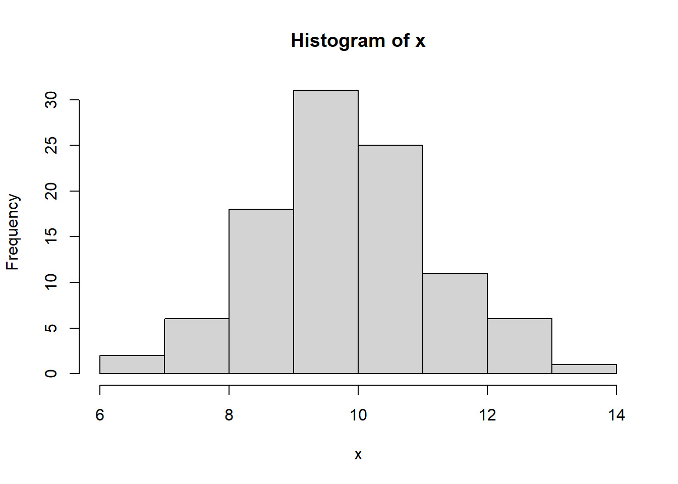
The Bernoulli and Binomial distributions are intimately related: a Binomial random variable corresponds to the number of successes in \(n\) independent Bernoulli trials. For example, consider flipping a coin. Each coin flip can be modelled as a Bernoulli\((p)\) random variable with probability of success (heads) equal to \(p\). If you flipped a coin \(n=10\) times and wanted to model the number of sucesses (heads) in \(n=10\) trials, that would be a Binomial(\(n,p\)) random variable.

R has four functions that can be used to compute both Bernoulli and Binomial probabilities: dbinom( ), pbinom( ), qbinom( ), rbinom( ).

dbinom(x,size,prob) probability mass function (PMF) - input: x is the number of successes, size is the number of trials \(n\), prob is the probability of success \(p\) - output: a probability since \(0\leq P(X=x)\leq1\) - example: evaluate \(P(X=x)\)

pbinom(q,size,prob) probability distribution function (CDF) - input: q is the value for which you want to find the area below/above, size is the number of trials \(n\), prob is the probability of success \(p\) - output: a probability - example: evaluate \(P(X\leq x)\)

qbinom(p,size,prob) quantile function
- input: p is a probability, size is the number of trials \(n\), prob is the probability of success \(p\) - output: a positive integer since \(X\in\{0,1,\dotsc,n\}\) - example: find \(q\) s.t. \(P(X\leq q)=p\)

rbinom(n,size,prob) random number generator
- input: n is the number of observations you want to generate, size is the number of trials \(n\), prob is the probability of success \(p\) - output: a vector of n positive integers - example: generate \(n\) independent Binomial\((n,p)\) random variables

Note: These functions correspond to the Bernoulli distribution whenever size=1.

More information is also accessible in R if you type ?dbinom, ?pbinom, ?qbinom, or ?rbinom.

2.2.1 Probability Mass Function (dbinom)

PROBLEM 13: If you flip a coin \(n=5\) times and in each flip the probability of heads is \(p=0.5\), what is the chance that you get 2 successes?

Solution:

Here, our random variable \(X\) is the number of successes in \(n\) independent trials, so \(X\sim\text{Binomial}(n,p)\) with \(n=5\) and \(p=0.5\).

dbinom(2, size=5, prob=0.5)

[1] 0.3125

We can also check our answer using the Binomial probability mass function: \(P(X=x)={n\choose x}p^x(1-p)^{n-x}\).

choose(5,2)*0.5^2*(1-0.5)^(5-2)

[1] 0.3125

2.2.2 Cumulative Distribution Function (pbinom)

PROBLEM 14: If you flip a coin \(n=5\) times and in each flip the probability of heads is \(p=0.5\), what is the chance that you get at most 2 successes?

Solution:

Now we want to find \(P(X\leq2)\). We know that \(P(X\leq2)=P(X=2)+P(X=1)+P(X=0)\), so we could again use the dbinom( ) function.

dbinom(2, size=5, prob=0.5) + dbinom(1, size=5, prob=0.5) + dbinom(0, size=5, prob=0.5)

[1] 0.5

The problem is that this approach becomes cumbersome as the number of trials increases. A more efficient approach is to recognize that \(P(X\leq2)\) takes the form of the CDF and use pnorm( ).

pbinom(2, size=5, prob=0.5)

[1] 0.5

PROBLEM 15: If you flip a coin \(n=100\) times and in each flip the probability of heads is \(p=0.25\), what is the chance that you get at most 20 successes?

Solution:

pbinom(20, size=100, prob=0.25)

[1] 0.1488311

PROBLEM 16: If you flip a coin \(n=100\) times and in each flip the probability of heads is \(p=0.25\), what is the chance that you get at least 20 successes?

Solution:

We have two ways to solve this problem. First, we can write \(P(X\geq 20)=1-P(X<20)=1-P(X\leq 19)\) where \(P(X<20)=P(X\leq 19)\) since \(X\) is discrete.

1-pbinom(19, size=100, prob=0.25)

[1] 0.9004696

Alternatively, we can use the lower.tail=FALSE option to tell R we want the probability greater than x. However, note that this is strictly greater than, so we must again remember than \(P(X\geq 20)=P(X>19)\).

pbinom(19, size=100, prob=0.25, lower.tail=FALSE)

[1] 0.9004696

2.2.3 Quantile Function (qbinom)

PROBLEM 17: Suppose you flip a coin \(n=20\) times where each flip has a probability of heads equal to \(p=0.5\). Find the value \(q\) such that the probability of getting at most \(q\) successes is equal to 0.25.

Solution:

qbinom(0.25, size=20, prob=0.5)

[1] 8

2.2.4 Random Number Generator (rbinom)

PROBLEM 18: Generate \(n=50\) Bernoulli\((p)\) random variables with \(p=0.2\).

Solution:

x = rbinom(50, size=1, prob=0.2)
x

 [1] 0 0 0 0 0 0 0 0 0 1 0 1 1 1 0 0 0 0 0 1 0 0 0 0 0 0 0 0 0 0 1 0 0 1 0 0 0 0
[39] 0 0 0 0 1 1 0 0 1 0 0 0

barplot(table(x))

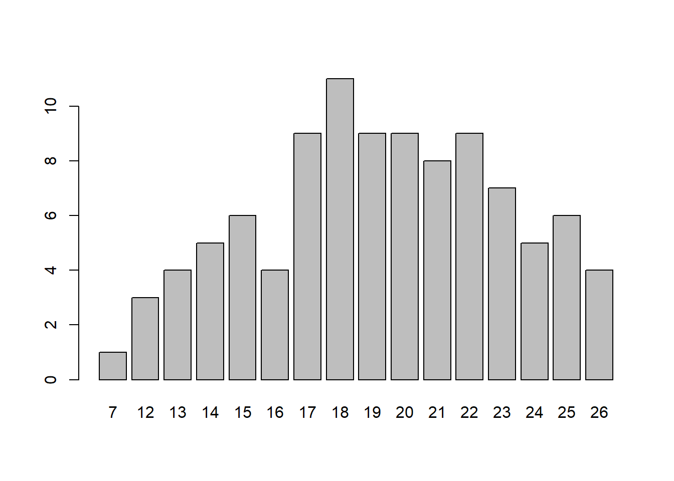
PROBLEM 19: Generate \(n=100\) Binomial\((n,p)\) random variables with \(p=0.4\).

Solution:

x = rbinom(100, size=100, prob=0.2)
x

  [1] 23 25 12 27 29 26 13 22 16 25 18 18 23 16 20 14 19 21 19 19 25 26 29 16 22
 [26] 19 22 17 19 27 20 24 18 22 18 23 18 16 21 20 24 20 17 17 18 17 20 21 21 14
 [51] 23 20 19 20 19 20 23 23 25 23 23 17 18 21 20 13 23 19 15 20 22 20 17 24 19
 [76] 17 18 21 24 20 19 24 29 21 17 13 14 20 27 18 23 20 25 16 24 22 29 24 21 15

barplot(table(x))